Ohm’s Law

Ohm’s Law Explained

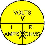
V, I, and R, the parameters of Ohm’s law

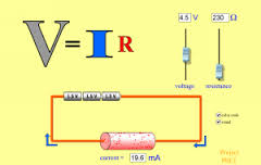
Ohm’s law states that the current through a conductor between two points is directlyproportional to the potential difference across the two points. Introducing the constant of proportionality, the resistance, one arrives at the usual mathematical equation that describes this relationship:

where I is the current through the conductor in units of amperes, V is the potential difference measured across the conductor in units of volts, and R is the resistance of the conductor in units of ohms. More specifically, Ohm’s law states that the R in this relation is constant, independent of the current.

The law was named after the German physicist Georg Ohm, who, in a treatise published in 1827, described measurements of applied voltage and current through simple electrical circuits containing various lengths of wire. He presented a slightly more complex equation than the one above (see History section below) to explain his experimental results. The above equation is the modern form of Ohm’s law.

In physics, the term Ohm’s law is also used to refer to various generalizations of the law originally formulated by Ohm. The simplest example of this is:

where J is the current density at a given location in a resistive material, E is the electric field at that location, and σ is a material dependent parameter called the conductivity. This reformulation of Ohm’s law is due to Gustav Kirchhoff.

History

In January 1781, before Georg Ohm‘s work, Henry Cavendish experimented with Leyden jars and glass tubes of varying diameter and length filled with salt solution. He measured the current by noting how strong a shock he felt as he completed the circuit with his body. Cavendish wrote that the “velocity” (current) varied directly as the “degree of electrification” (voltage). He did not communicate his results to other scientists at the time, and his results were unknown until Maxwell published them in 1879.

Ohm did his work on resistance in the years 1825 and 1826, and published his results in 1827 as the book Die galvanische Kette, mathematisch bearbeitet (The galvanic circuit investigated mathematically).  He drew considerable inspiration from Fourier‘s work on heat conduction in the theoretical explanation of his work. For experiments, he initially used voltaic piles, but later used at hermocouple as this provided a more stable voltage source in terms of internal resistance and constant potential difference. He used a galvanometer to measure current, and knew that the voltage between the thermocouple terminals was proportional to the junction temperature. He then added test wires of varying length, diameter, and material to complete the circuit. He found that his data could be modeled through the equation

where x was the reading from the galvanometer, l was the length of the test conductor, a depended only on the thermocouple junction temperature, and b was a constant of the entire setup. From this, Ohm determined his law of proportionality and published his results.

Ohm’s law was probably the most important of the early quantitative descriptions of the physics of electricity. We consider it almost obvious today. When Ohm first published his work, this was not the case; critics reacted to his treatment of the subject with hostility. They called his work a “web of naked fancies” and the German Minister of Education proclaimed that “a professor who preached such heresies was unworthy to teach science.”  The prevailing scientific philosophy in Germany at the time asserted that experiments need not be performed to develop an understanding of nature because nature is so well ordered, and that scientific truths may be deduced through reasoning alone.  Also, Ohm’s brother Martin, a mathematician, was battling the German educational system. These factors hindered the acceptance of Ohm’s work, and his work did not become widely accepted until the 1840’s. Fortunately, Ohm received recognition for his contributions to science well before he died.

In the 1850’s, Ohm’s law was known as such and was widely considered proved, and alternatives, such as “Barlow’s law“, were discredited, in terms of real applications to telegraph system design, as discussed by Samuel F. B. Morse in 1855.

While the old term for electrical conductance, the mho (the inverse of the resistance unit ohm), is still used, a new name, the siemens, was adopted in 1971, honoring Ernst Werner von Siemens. The siemens is preferred in formal papers.

In the 1920s, it was discovered that the current through an ideal resistor actually has statistical fluctuations, which depend on temperature, even when voltage and resistance are exactly constant; this fluctuation, now known as Johnson–Nyquist noise, is due to the discrete nature of charge. This thermal effect implies that measurements of current and voltage that are taken over sufficiently short periods of time will yield ratios of V/I that fluctuate from the value of R implied by the time average or ensemble average of the measured current; Ohm’s law remains correct for the average current, in the case of ordinary resistive materials.

Ohm’s work long preceded Maxwell’s equations and any understanding of frequency-dependent effects in AC circuits. Modern developments in electromagnetic theory and circuit theory do not contradict Ohm’s law when they are evaluated within the appropriate limits.

Scope

Ohm’s law is an empirical law, a generalization from many experiments that have shown that current is approximately proportional to electric field for most materials. It is less fundamental than Maxwell’s equations and is not always obeyed. Any given material will break down under a strong-enough electric field, and some materials of interest in electrical engineering are “non-ohmic” under weak fields.

Ohm’s law has been observed on a wide range of length scales. In the early 20th century, it was thought that Ohm’s law would fail at the atomic scale, but experiments have not borne out this expectation. As of 2012, researchers have demonstrated that Ohm’s law works for silicon wires as small as four atoms wide and one atom high.

Microscopic origins

The dependence of the current density on the applied electric field is essentially quantum mechanical in nature; (see Classical and quantum conductivity).  A qualitative description leading to Ohm’s law can be based upon classical mechanics using the Drude model developed by Paul Drude in 1900.

The Drude model treats electrons (or other charge carriers) like pinballs bouncing among the ions that make up the structure of the material. Electrons will be accelerated in the opposite direction to the electric field by the average electric field at their location. With each collision, though, the electron is deflected in a random direction with a velocity that is much larger than the velocity gained by the electric field. The net result is that electrons take a zigzag path due to the collisions, but generally drift in a direction opposing the electric field.

The drift velocity then determines the electric current density and its relationship to E and is independent of the collisions. Drude calculated the average drift velocity from p = −e Eτ where p is the average momentum, −e is the charge of the electron and τ is the average time between the collisions. Since both the momentum and the current density are proportional to the drift velocity, the current density becomes proportional to the applied electric field; this leads to Ohm’s law.

Hydraulic analogy

A hydraulic analogy is sometimes used to describe Ohm’s law. Water pressure, measured by pascals (or PSI), is the analog of voltage because establishing a water pressure difference between two points along a (horizontal) pipe causes water to flow. Water flow rate, as in liters per second, is the analog of current, as in coulombs per second. Finally, flow restrictors—such as apertures placed in pipes between points where the water pressure is measured—are the analog of resistors. We say that the rate of water flow through an aperture restrictor is proportional to the difference in water pressure across the restrictor. Similarly, the rate of flow of electrical charge, that is, the electric current, through an electrical resistor is proportional to the difference in voltage measured across the resistor.

Flow and pressure variables can be calculated in fluid flow network with the use of the hydraulic ohm analogy.  The method can be applied to both steady and transient flow situations. In the linear laminar flow region, Poiseuille’s law describes the hydraulic resistance of a pipe, but in the turbulent flow region the pressure–flow relations become nonlinear.

The hydraulic analogy to Ohm’s law has been used, for example, to approximate blood flow through the circulatory system.

Circuit analysis

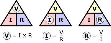
In circuit analysis, three equivalent expressions of Ohm’s law are used interchangeably:

Each equation is quoted by some sources as the defining relationship of Ohm’s law, or all three are quoted, or derived from a proportional form, or even just the two that do not correspond to Ohm’s original statement may sometimes be given.

The interchangeability of the equation may be represented by a triangle, where V (voltage) is placed on the top section, the I (current) is placed to the left section, and the R (resistance) is placed to the right. The line that divides the left and right sections indicate multiplication, and the divider between the top and bottom sections indicates division (hence the division bar).

Resistive circuits

Resistors are circuit elements that impede the passage of electric charge in agreement with Ohm’s law, and are designed to have a specific resistance value R. In a schematic diagram the resistor is shown as a zig-zag symbol. An element (resistor or conductor) that behaves according to Ohm’s law over some operating range is referred to as an ohmic device (or an ohmic resistor) because Ohm’s law and a single value for the resistance suffice to describe the behavior of the device over that range.

Ohm’s law holds for circuits containing only resistive elements (no capacitances or inductances) for all forms of driving voltage or current, regardless of whether the driving voltage or current is constant (DC) or time-varying such as AC. At any instant of time Ohm’s law is valid for such circuits.

Resistors which are in series or in parallel may be grouped together into a single “equivalent resistance” in order to apply Ohm’s law in analyzing the circuit. This application of Ohm’s law is illustrated with examples in “How To Analyze Resistive Circuits Using Ohm’s Law” on wikiHow.

Reactive circuits with time-varying signals

When reactive elements such as capacitors, inductors, or transmission lines are involved in a circuit to which AC or time-varying voltage or current is applied, the relationship between voltage and current becomes the solution to a differential equation, so Ohm’s law (as defined above) does not directly apply since that form contains only resistances having value R, not complex impedances which may contain capacitance (“C”) or inductance (“L”).

Equations for time-invariant AC circuits take the same form as Ohm’s law, however, the variables are generalized to complex numbers and the current and voltage waveforms are complex exponentials.

In this approach, a voltage or current waveform takes the form , where t is time, s is a complex parameter, and A is a complex scalar. In any linear time-invariant system, all of the currents and voltages can be expressed with the same s parameter as the input to the system, allowing the time-varying complex exponential term to be canceled out and the system described algebraically in terms of the complex scalars in the current and voltage waveforms.

The complex generalization of resistance is impedance, usually denoted Z; it can be shown that for an inductor,

and for a capacitor,

We can now write,

where V and I are the complex scalars in the voltage and current respectively and Z is the complex impedance.

This form of Ohm’s law, with Z taking the place of R, generalizes the simpler form. When Z is complex, only the real part is responsible for dissipating heat.

In the general AC circuit, Z varies strongly with the frequency parameter s, and so also will the relationship between voltage and current.

For the common case of a steady sinusoid, the s parameter is taken to be , corresponding to a complex sinusoid . The real parts of such complex current and voltage waveforms describe the actual sinusoidal currents and voltages in a circuit, which can be in different phases due to the different complex scalars.

https://en.wikipedia.org/wiki/Ohm’s_law